Riemannian BCI
Signal processing in covariance matrices space
The most successful approaches in feature extraction and signal processing for BCI, i.e. those providing the highest transfer rates and the most robust representations, share one common ground: they are all estimating the covariance from the signal to build or to derive their feature. The covariance captures the degree of linear dependence between several random variables, that is, how the brain signals change relatively to each other. If two signals show the same variations, increasing and decreasing at the same time, they are dependent. The notion of covariance is central in several fields of science, such as mathematical finance, meteorology, oceanography, and, of course, signal processing. A correct covariance estimation requires to take into account a noticeable part of the time signal history. This fact has a strong impact when setting up a BCI system, as it introduces a delay to allow a correct processing and interpretation of the brain signal. Special attention is thus needed when dealing with covariance-based approaches in online systems, to aim for a robust system without impeding the interactions with a high latency.
The Riemannian BCI techniques have demonstrated their benefit on several occasions, leading to winning algorithms in international competitions and to state-of-the-art results on renowned benchmarks.
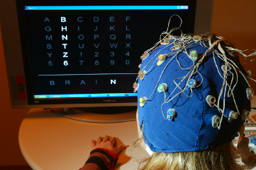
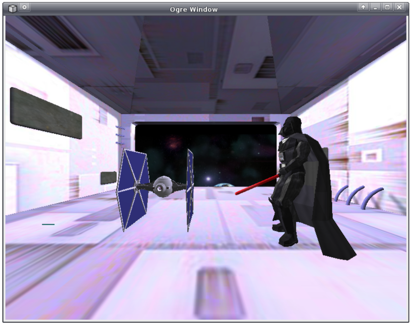
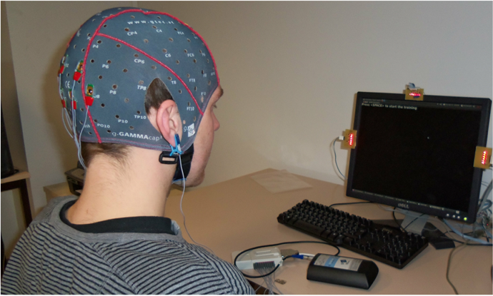
Classical machine learning pipeline involves 3 steps:
- Offline model selection: pick best preprocessing and classifier couple
- Calibration: Optimize spatial filter for subject’s current session
- Training: train classifier on preprocessed calibration data
- New session: Repeat from (2)
All efficient approaches try to find a spatial filter \(W_d \in \mathbb{R}^{C \times D}\), where \(C\) is the number of channels and \(D \leqslant C\) such that \(W^TX\) maximizes the SNR. The ideas are twofold: build in a surrogate space, where the channels are reweighted to enhance the signal of interest, and reduce the dimensionality as the EEG signal is highly correlated. But these approaches are efficient only on clean datasets and with a lengthy calibration phase, that is prone to overfitting. Still, these approaches fail for 20% of the subjects as it could be seen from the results of international competition.
Covariance-based methods are nested in all the above-mentioned approaches for processing EEG signal in BCI. While covariance matrices have a specific non-flat geometry, most of the common approaches rely on Euclidean techniques.
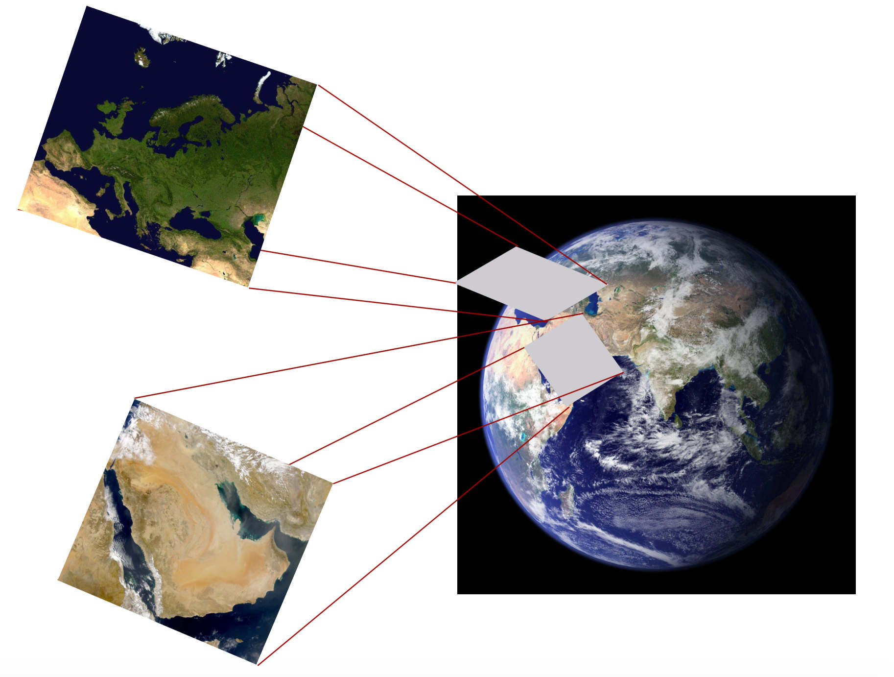
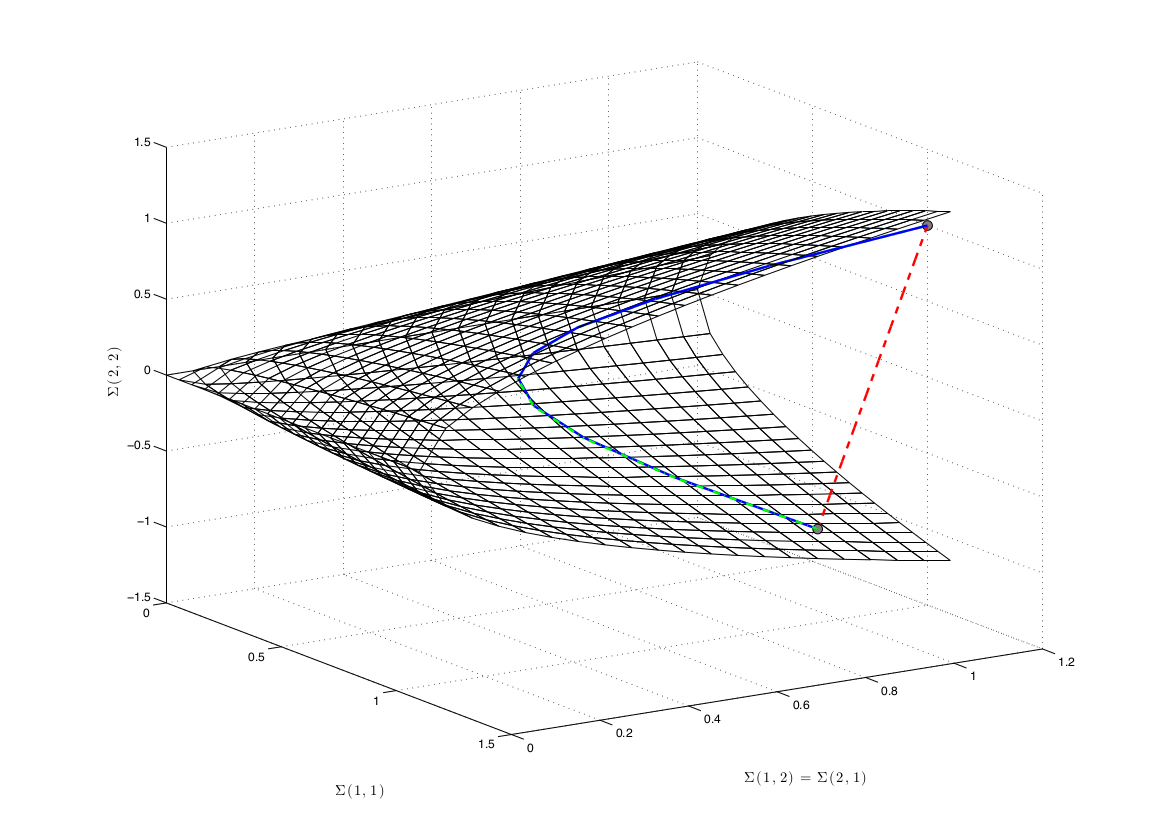
Covariance matrices are as elements of the manifold of symmetric and positive-definite matrices : \(\mathcal{M}_C = \left\{ \Sigma \in \mathbb{R}^{C \times C} : \Sigma = \Sigma^T \text{and} x^T \Sigma x > 0, \forall x \in \mathbb{R}^C \backslash 0 \right\}\). Combined with a proper distance, such as the affine-invariant distance \(d(\Sigma_1, \Sigma_2) = || \log(\Sigma_1^{-\frac{1}{2}} \Sigma_2 \Sigma_1^{-\frac{1}{2}}) ||_F\), this defines a Riemannian manifold.
From the BCI perspective, the most interesting points regarding this Riemannian geometry are the invariance provided by the chosen distance. There is many possible choices described in the literature [1], each one coming with specific invariances. The affine-invariant distance (or Fisher metric) endows the distance with the invariance to affine transforms, as suggested by its name : \(d(\Sigma_1, \Sigma_2) = d(W^T \Sigma_1 W, W^T \Sigma_2 W)\). This means that when measuring the distance between two EEG signals (seen as covariance matrices), this distance is not sensitive to any reweighting of channels. It is like always working with the optimal spatial filter \(W\)!
Most of the classical machine learning algorithms are working only in Euclidean spaces, but some of them could be adapted to take into account the geometry of the covariance space. This is the case for the minimum distance to mean (MDM) or any classical machine learning classifiers applied in tangent space.
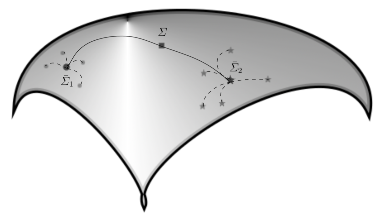
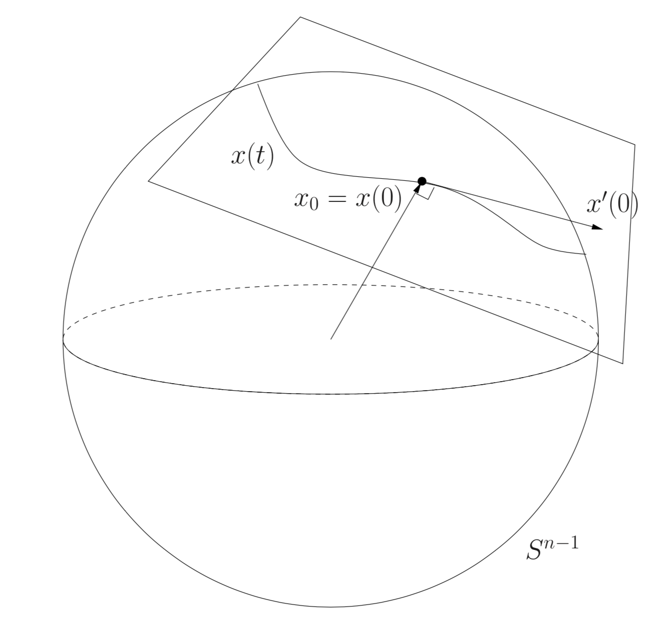
These classifiers yield state-of-the-art results for BCI [2], [3]
| P300 - Brain Invaders | SSVEP - Exoskeleton | MI - BCI IV 2a |
|---|---|---|
| MDM - 89.04% ± 8.79 | MDM - 89.85% ± 8.0 | TSLDA - 70.2% ± 17.1 |
| SWLDA - 86.08% ± 10.05 | CCA - 87.50% ± 15.1 | CSPLDA - 65.1% ± 17.9 |
| XDAWN - 86.26% ±9.96 | FBCCA - 87.40% ± 15.7 | SVM - 63.2% ± 15.2 |
In order to compare existing algorithms, a framework called MOABB allows to download EEG datasets and to evaluate existing classifiers in a few lines of Python. Testing MDM classifier on data from the BCI Competition IV and from paper from Zhou et al is simple as:
datasets = [BNCI2014001(), Zhou2016()]
paradigm = LeftRightImagery()
pipeline = {'MDM': make_pipeline(Covariances('oas'), MDM(metric='riemann'))}
evaluation = WithinSessionEvaluation(paradigm=paradigm, datasets=datasets, overwrite=True)
results = evaluation.process(pipelines)
More complete examples are available as notebooks from the MOABB workshop in Graz 2019.
References
[1] S. Chevallier, E. K. Kalunga, Q. Barthélemy, E. Monacelli. “Review of Riemannian distances and divergences applied to SSVEP-based BCI”, Neuroinformatics, TBP.
[2] M. Congedo, A. Barachant, A. Andreev ,”A New generation of Brain-Computer Interface Based on Riemannian Geometry”, arXiv: 1310.8115, 2013.
[3] E. K. Kalunga, S. Chevallier, Q. Barthélemy, K. Djouani, E. Monacelli, Y. Hamam, “Online SSVEP-based BCI using Riemannian geometry”, Neurocomputing, vol. 191, p. 55-68, 2016.